머신러닝
Linear Regression
J.H_DA
2022. 4. 15. 16:36
#### sklearn.linear_model.LinearRegression
class sklearn.linear_model.LinearRegression(*, fit_intercept=True, normalize='deprecated', copy_X=True, n_jobs=None, positive=False)
linear Regression 은 예측값과 실제 값의 RSS를 최소호해 OLS 추정 방식으로 구현한 클래스이다.
선형 회귀 의 다중 공선성 문제
일반적으로 선형 회귀는 입력 피처의 독립성에 많은 영향을 받는다. 이러한 현상을 다중공선성 문제라고 하며 일반적으로 상관관계가 높은 피처가 많은 경우 독립적인 중요한 피처만 남기고 제거하거나 규제를 적용한다.
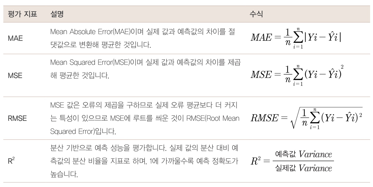
회귀 평가 지표
sklearn.linear_model.LinearRegression
- class sklearn.linear_model.LinearRegression(*, fit_intercept=True, normalize='deprecated', copy_X=True, n_jobs=None, positive=False)
linear Regression 은 예측값과 실제 값의 RSS를 최소호해 OLS 추정 방식으로 구현한 클래스이다.
선형 회귀 예제
In [10]:
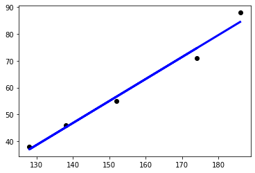
# 인간의 키와 몸무게의 선형 회귀 학습

import matplotlib.pylab as plt
from sklearn import linear_model

reg = linear_model.LinearRegression()

X=[[174],[152], [138], [128],[186]]
y=[71,55,46,38,88]
reg.fit(X,y)

print(reg.predict([[175]]))

# 학습 데이터와 y값을 산포도로 그린다.
plt.scatter(X,y, color ='black')

# 학습 데이터를 입력으로 하여 예측값을 계산한다.
y_pred = reg.predict(X)

## 학습 데이터와 예측값으로 선그래프로 그린다.
## 계산된 기울기와 y 절편을 가지는 직선이 그려진다.
plt.plot(X,y_pred, color='blue', linewidth=3)
plt.show()
[75.51209952]
In [8]:
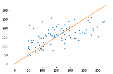
# 당뇨병 예제
import matplotlib.pylab as plt
import numpy as np
from sklearn.linear_model import LinearRegression
from sklearn import datasets
from sklearn.model_selection import train_test_split

diabetes=datasets.load_diabetes()


X_train, X_test, y_train, y_test = train_test_split(diabetes.data,diabetes.target, test_size=0.2, random_state=0)

model = LinearRegression()
model.fit(X_train, y_train)

y_pred = model.predict(X_test)

plt.plot(y_test, y_pred,'.')


# 직석을 그리기 위하여 완벽한 선형 데이터 생성
x=np.linspace(0,330,100)
y=x
plt.plot(x,y)
plt.show()
보스턴 주택 가격 예측
In [56]:
## 과제1
import numpy as np
import matplotlib.pyplot as plt
import pandas as pd
import seaborn as sns
from scipy import stats
from sklearn.datasets import load_boston
from pandas import read_csv
%matplotlib inline

column_names = ['CRIM', 'ZN', 'INDUS', 'CHAS', 'NOX', 'RM', 'AGE', 'DIS', 'RAD', 'TAX', 'PTRATIO', 'B', 'LSTAT', 'PRICE']
bostonDF = read_csv('./housing.csv', header=None, delimiter=r"\s+", names=column_names)
print(bostonDF.head(5))
      CRIM    ZN  INDUS  CHAS    NOX     RM   AGE     DIS  RAD    TAX  \
0  0.00632  18.0   2.31     0  0.538  6.575  65.2  4.0900    1  296.0
1  0.02731   0.0   7.07     0  0.469  6.421  78.9  4.9671    2  242.0
2  0.02729   0.0   7.07     0  0.469  7.185  61.1  4.9671    2  242.0
3  0.03237   0.0   2.18     0  0.458  6.998  45.8  6.0622    3  222.0
4  0.06905   0.0   2.18     0  0.458  7.147  54.2  6.0622    3  222.0

   PTRATIO       B  LSTAT  PRICE
0     15.3  396.90   4.98   24.0
1     17.8  396.90   9.14   21.6
2     17.8  392.83   4.03   34.7
3     18.7  394.63   2.94   33.4
4     18.7  396.90   5.33   36.2
In [57]:
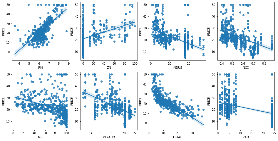
# 2개의 행과 4개의 열을 가진 subplots를 이용. axs는 4x2개의 ax를 가짐.
fig, axs = plt.subplots(figsize=(16,8) , ncols=4 , nrows=2)
lm_features = ['RM','ZN','INDUS','NOX','AGE','PTRATIO','LSTAT','RAD']
for i , feature in enumerate(lm_features):
    row = int(i/4)
    col = i%4
    # 시본의 regplot을 이용해 산점도와 선형 회귀 직선을 함께 표현
    sns.regplot(x=feature , y='PRICE',data=bostonDF , ax=axs[row][col])
In [58]:
# 학습과 테스트 데이터 세트로 분리하고 학습/예측/평가 수행
from sklearn.model_selection import train_test_split
from sklearn.linear_model import LinearRegression
from sklearn.metrics import mean_squared_error , r2_score
from sklearn.metrics import accuracy_score

y_target = bostonDF['PRICE']
X_data = bostonDF.drop(['PRICE'],axis=1,inplace=False)

X_train , X_test , y_train , y_test = train_test_split(X_data , y_target ,test_size=0.3, random_state=156)

# Linear Regression OLS로 학습/예측/평가 수행.
lr = LinearRegression()
lr.fit(X_train ,y_train)
y_preds = lr.predict(X_test)
mse = mean_squared_error(y_test, y_preds)
rmse = np.sqrt(mse)

lr_accuracy= lr.score(X_train, y_train)

print('정확도: {0:.4f}'.format(lr_accuracy))
print('MSE : {0:.3f} , RMSE : {1:.3F}'.format(mse , rmse))
print('Variance score : {0:.3f}'.format(r2_score(y_test, y_preds)))
정확도: 0.7274
MSE : 17.297 , RMSE : 4.159
Variance score : 0.757
Polynomial Regression
In [60]:
from sklearn.preprocessing import PolynomialFeatures
import numpy as np

# 다항식으로 변환한 단항식 생성, [[0,1],[2,3]]의 2X2 행렬 생성
X = np.arange(4).reshape(2,2)
print('일차 단항식 계수 feature:\n',X )

# degree = 2 인 2차 다항식으로 변환하기 위해 PolynomialFeatures를 이용하여 변환
poly = PolynomialFeatures(degree=2)
poly.fit(X)
poly_ftr = poly.transform(X)
print('변환된 2차 다항식 계수 feature:\n', poly_ftr)
일차 단항식 계수 feature:
 [[0 1]
 [2 3]]
변환된 2차 다항식 계수 feature:
 [[1. 0. 1. 0. 0. 1.]
 [1. 2. 3. 4. 6. 9.]]
In [61]:
# 3차 다항식 결정값을 구하는 함수 생성
def polynomial_func(X):
    y = 1 + 2*X[:,0] + 3*X[:,0]**2 + 4*X[:,1]**3
    return y

X = np.arange(0,4).reshape(2,2)

print('일차 단항식 계수 feature: \n' ,X)
y = polynomial_func(X)
print('삼차 다항식 결정값: \n', y)

# 3 차 다항식 변환
poly_ftr = PolynomialFeatures(degree=3).fit_transform(X)
print('3차 다항식 계수 feature: \n',poly_ftr)

# Linear Regression에 3차 다항식 계수 feature와 3차 다항식 결정값으로 학습 후 회귀 계수 확인
model = LinearRegression()
model.fit(poly_ftr,y)
print('Polynomial 회귀 계수\n' , np.round(model.coef_, 2))
print('Polynomial 회귀 Shape :', model.coef_.shape)
일차 단항식 계수 feature:
 [[0 1]
 [2 3]]
삼차 다항식 결정값:
 [  5 125]
3차 다항식 계수 feature:
 [[ 1.  0.  1.  0.  0.  1.  0.  0.  0.  1.]
 [ 1.  2.  3.  4.  6.  9.  8. 12. 18. 27.]]
Polynomial 회귀 계수
 [0.   0.18 0.18 0.36 0.54 0.72 0.72 1.08 1.62 2.34]
Polynomial 회귀 Shape : (10,)
In [62]:
# 파이프라인 이용 다항 회귀
from sklearn.preprocessing import PolynomialFeatures
from sklearn.linear_model import LinearRegression
from sklearn.pipeline import Pipeline
import numpy as np

def polynomial_func(X):
    y = 1 + 2*X[:,0] + 3*X[:,0]**2 + 4*X[:,1]**3
    return y

# Pipeline 객체로 Streamline 하게 Polynomial Feature변환과 Linear Regression을 연결
model = Pipeline([('poly', PolynomialFeatures(degree=3)),
                  ('linear', LinearRegression())])
X = np.arange(4).reshape(2,2)
y = polynomial_func(X)

model = model.fit(X, y)
print('Polynomial 회귀 계수\n', np.round(model.named_steps['linear'].coef_, 2))
Polynomial 회귀 계수
 [0.   0.18 0.18 0.36 0.54 0.72 0.72 1.08 1.62 2.34]
In [63]:
# 다항 회귀를 이용한 보스턴 주택 가격 예측
from sklearn.model_selection import train_test_split
from sklearn.linear_model import LinearRegression
from sklearn.metrics import mean_squared_error , r2_score
from sklearn.preprocessing import PolynomialFeatures
from sklearn.linear_model import LinearRegression
from sklearn.pipeline import Pipeline
import numpy as np

# boston 데이타셋 로드
boston = load_boston()

# boston 데이타셋 DataFrame 변환
bostonDF = pd.DataFrame(boston.data , columns = boston.feature_names)

# boston dataset의 target array는 주택 가격임. 이를 PRICE 컬럼으로 DataFrame에 추가함.
bostonDF['PRICE'] = boston.target
print('Boston 데이타셋 크기 :',bostonDF.shape)

y_target = bostonDF['PRICE']
X_data = bostonDF.drop(['PRICE'],axis=1,inplace=False)


X_train , X_test , y_train , y_test = train_test_split(X_data , y_target ,test_size=0.3, random_state=156)

## Pipeline을 이용하여 PolynomialFeatures 변환과 LinearRegression 적용을 순차적으로 결합.
p_model = Pipeline([('poly', PolynomialFeatures(degree=3, include_bias=False)),
                  ('linear', LinearRegression())])

p_model.fit(X_train, y_train)
y_preds = p_model.predict(X_test)
mse = mean_squared_error(y_test, y_preds)
rmse = np.sqrt(mse)


print('MSE : {0:.3f} , RMSE : {1:.3F}'.format(mse , rmse))
print('Variance score : {0:.3f}'.format(r2_score(y_test, y_preds)))
Boston 데이타셋 크기 : (506, 14)
MSE : 79625.593 , RMSE : 282.180
Variance score : -1116.598
C:\ProgramData\Anaconda3\lib\site-packages\sklearn\utils\deprecation.py:87: FutureWarning: Function load_boston is deprecated; `load_boston` is deprecated in 1.0 and will be removed in 1.2.

    The Boston housing prices dataset has an ethical problem. You can refer to
    the documentation of this function for further details.

    The scikit-learn maintainers therefore strongly discourage the use of this
    dataset unless the purpose of the code is to study and educate about
    ethical issues in data science and machine learning.

    In this special case, you can fetch the dataset from the original
    source::

        import pandas as pd
        import numpy as np


        data_url = "http://lib.stat.cmu.edu/datasets/boston"
        raw_df = pd.read_csv(data_url, sep="\s+", skiprows=22, header=None)
        data = np.hstack([raw_df.values[::2, :], raw_df.values[1::2, :2]])
        target = raw_df.values[1::2, 2]

    Alternative datasets include the California housing dataset (i.e.
    :func:`~sklearn.datasets.fetch_california_housing`) and the Ames housing
    dataset. You can load the datasets as follows::

        from sklearn.datasets import fetch_california_housing
        housing = fetch_california_housing()

    for the California housing dataset and::

        from sklearn.datasets import fetch_openml
        housing = fetch_openml(name="house_prices", as_frame=True)

    for the Ames housing dataset.

  warnings.warn(msg, category=FutureWarning)
In [64]:
X_train_poly= PolynomialFeatures(degree=2, include_bias=False).fit_transform(X_train, y_train)
X_train_poly.shape, X_train.shape
Out[64]:
((354, 104), (354, 13))Polynomial Regression 을 이용한 Underfitting, Overfitting 이해
In [65]:
import numpy as np
import matplotlib.pyplot as plt
from sklearn.pipeline import Pipeline
from sklearn.preprocessing import PolynomialFeatures
from sklearn.linear_model import LinearRegression
from sklearn.model_selection import cross_val_score
%matplotlib inline

# random 값으로 구성된 X값에 대해 Cosine 변환값을 반환.
def true_fun(X):
    return np.cos(1.5 * np.pi * X)

# X는 0 부터 1까지 30개의 random 값을 순서대로 sampling 한 데이타 입니다.
np.random.seed(0)
n_samples = 30
X = np.sort(np.random.rand(n_samples))

# y 값은 cosine 기반의 true_fun() 에서 약간의 Noise 변동값을 더한 값입니다.
y = true_fun(X) + np.random.randn(n_samples) * 0.1


plt.scatter(X, y)
Out[65]:
<matplotlib.collections.PathCollection at 0x22fceb08640>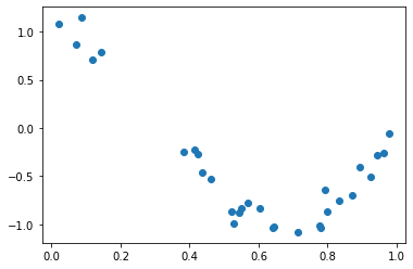
In [66]:
plt.figure(figsize=(14, 5))
degrees = [1, 4, 15]

# 다항 회귀의 차수(degree)를 1, 4, 15로 각각 변화시키면서 비교합니다.
for i in range(len(degrees)):
    ax = plt.subplot(1, len(degrees), i + 1)
    plt.setp(ax, xticks=(), yticks=())

    # 개별 degree별로 Polynomial 변환합니다.
    polynomial_features = PolynomialFeatures(degree=degrees[i], include_bias=False)
    linear_regression = LinearRegression()
    pipeline = Pipeline([("polynomial_features", polynomial_features),
                         ("linear_regression", linear_regression)])
    pipeline.fit(X.reshape(-1, 1), y)

    # 교차 검증으로 다항 회귀를 평가합니다.
    scores = cross_val_score(pipeline, X.reshape(-1,1), y,scoring="neg_mean_squared_error", cv=10)
    coefficients = pipeline.named_steps['linear_regression'].coef_
    print('\nDegree {0} 회귀 계수는 {1} 입니다.'.format(degrees[i], np.round(coefficients),2))
    print('Degree {0} MSE 는 {1:.2f} 입니다.'.format(degrees[i] , -1*np.mean(scores)))

    # 0 부터 1까지 테스트 데이터 세트를 100개로 나눠 예측을 수행합니다.
    # 테스트 데이터 세트에 회귀 예측을 수행하고 예측 곡선과 실제 곡선을 그려서 비교합니다.
    X_test = np.linspace(0, 1, 100)
    # 예측값 곡선
    plt.plot(X_test, pipeline.predict(X_test[:, np.newaxis]), label="Model")
    # 실제 값 곡선
    plt.plot(X_test, true_fun(X_test), '--', label="True function")
    plt.scatter(X, y, edgecolor='b', s=20, label="Samples")

    plt.xlabel("x"); plt.ylabel("y"); plt.xlim((0, 1)); plt.ylim((-2, 2)); plt.legend(loc="best")
    plt.title("Degree {}\nMSE = {:.2e}(+/- {:.2e})".format(degrees[i], -scores.mean(), scores.std()))

plt.show()
Degree 1 회귀 계수는 [-2.] 입니다.
Degree 1 MSE 는 0.41 입니다.

Degree 4 회귀 계수는 [  0. -18.  24.  -7.] 입니다.
Degree 4 MSE 는 0.04 입니다.

Degree 15 회귀 계수는 [-2.98300000e+03  1.03900000e+05 -1.87417100e+06  2.03717220e+07
 -1.44873987e+08  7.09318780e+08 -2.47066977e+09  6.24564048e+09
 -1.15677067e+10  1.56895696e+10 -1.54006776e+10  1.06457788e+10
 -4.91379977e+09  1.35920330e+09 -1.70381654e+08] 입니다.
Degree 15 MSE 는 182815433.48 입니다.
728x90