### 차원 축소
- 학습 데이터 크기를 줄여서 학습 시간 절약
- 불필요한 피처들을 줄여서 모델 성능 향상에 기여
- 다차원의 데이터를 3차원 이하의 차원 축소를 통해서 시각적으로 보다 쉽게 데이터 패턴 인지
피처 선택: 특정 피처에 종속성이 강한 불피요한 피처는 아예 제거하고, 데이터의 특징을 잘 나타내는 주요 피처만 선택
피처 추출: 기존 피처를 저차원의 중요 피처로 압축해서 추출하는 것
피처 추출은 기존 피처를 단순 압축이 아닌, 피처를 함축적으로 더 잘 설명할 수 있는 또 라느 공간으로 매핑해 추출하는 것
PCA: 고차원의 원본 데이터를 저 차원의 부분 공간으로 투영하여 데이터를 축소하는 기법
PCA는 원본 데이터가 가지는 데이터 변동성을 가장 중요한 정보로 간주하며 이 변동성에 기반한 원본 데이터 투영으로 차원 축소를 진행
PCA를 선형대수 관점에서 해석해 보면, 입력 데이터의 공분산 행렬(Covariance Matrix)을 고유값 분해 하고, 이렇게 구한 고유벡터에 입력 데이터를 선형 변환하는 것이다.
공분산 구하고-> 고유벡터 구하기
* 고유벡터는 PCA의 주성분 벡터로서 입력 데이터의 분산이 큰 방향을 나타낸다.
* 고윳값은 바로 이 고유벡터의 크기를 나타내며, 동시에 입력 데이터의 분산을 나타낸다.
공분산 Cov(X, Y) > 0 은 X가 증가할때 Y 도 증가한다는 의미이다.
1. 공분산
In [34]:
import pandas as pd
import numpy as np
import matplotlib.pyplot as plt
import seaborn as sns

import warnings
warnings.filterwarnings('ignore', category= RuntimeWarning)

# Eating, exercise habbit and their body shape
df = pd.DataFrame(columns=['calory', 'breakfast', 'lunch', 'dinner', 'exercise', 'body_shape'])

df.loc[0] = [1200, 1, 0, 0, 2, 'Skinny']
df.loc[1] = [2800, 1, 1, 1, 1, 'Normal']
df.loc[2] = [3500, 2, 2, 1, 0, 'Fat']
df.loc[3] = [1400, 0, 1, 0, 3, 'Skinny']
df.loc[4] = [5000, 2, 2, 2, 0, 'Fat']
df.loc[5] = [1300, 0, 0, 1, 2, 'Skinny']
df.loc[6] = [3000, 1, 0, 1, 1, 'Normal']
df.loc[7] = [4000, 2, 2, 2, 0, 'Fat']
df.loc[8] = [2600, 0, 2, 0, 0, 'Normal']
df.loc[9] = [3000, 1, 2, 1, 1, 'Fat']
In [35]:
 y_target= df["body_shape"]
 X_train = df.drop(["body_shape"], axis=1)
In [36]:
from sklearn. preprocessing import StandardScaler
X_std = StandardScaler().fit_transform(X_train)
In [37]:
X_std
Out[37]:
array([[-1.35205803,  0.        , -1.3764944 , -1.28571429,  1.        ],
       [ 0.01711466,  0.        , -0.22941573,  0.14285714,  0.        ],
       [ 0.61612771,  1.29099445,  0.91766294,  0.14285714, -1.        ],
       [-1.18091145, -1.29099445, -0.22941573, -1.28571429,  2.        ],
       [ 1.89972711,  1.29099445,  0.91766294,  1.57142857, -1.        ],
       [-1.26648474, -1.29099445, -1.3764944 ,  0.14285714,  1.        ],
       [ 0.18826125,  0.        , -1.3764944 ,  0.14285714,  0.        ],
       [ 1.04399418,  1.29099445,  0.91766294,  1.57142857, -1.        ],
       [-0.15403193, -1.29099445,  0.91766294, -1.28571429, -1.        ],
       [ 0.18826125,  0.        ,  0.91766294,  0.14285714,  0.        ]])
1.1 Covariance Matrix of Features
In [38]:
import numpy as np

features = X_std.T
covarinace_matrix = np.cov(features)
covarinace_matrix
Out[38]:
array([[ 1.11111111,  0.88379717,  0.76782385,  0.89376551, -0.93179808],
       [ 0.88379717,  1.11111111,  0.49362406,  0.81967902, -0.71721914],
       [ 0.76782385,  0.49362406,  1.11111111,  0.40056715, -0.76471911],
       [ 0.89376551,  0.81967902,  0.40056715,  1.11111111, -0.63492063],
       [-0.93179808, -0.71721914, -0.76471911, -0.63492063,  1.11111111]])
1.2 고유벡터 와 고윳값 with 공분산 행렬
In [39]:
eig_vals, eig_vecs = np.linalg.eig(covarinace_matrix)
In [40]:
eig_vals
Out[40]:
array([4.0657343 , 0.8387565 , 0.07629538, 0.27758568, 0.2971837 ])In [41]:
eig_vecs
Out[41]:
array([[-0.508005  , -0.0169937 , -0.84711404,  0.11637853,  0.10244985],
       [-0.44660335, -0.36890361,  0.12808055, -0.63112016, -0.49973822],
       [-0.38377913,  0.70804084,  0.20681005, -0.40305226,  0.38232213],
       [-0.42845209, -0.53194699,  0.3694462 ,  0.22228235,  0.58954327],
       [ 0.46002038, -0.2816592 , -0.29450345, -0.61341895,  0.49601841]])
In [42]:
eig_vals[0]/sum(eig_vals)
Out[42]:
0.73183217314275441.3 project data into selected
In [43]:
projected_x = X_std.dot(eig_vecs.T[0]) # T transpose 행과 열을 바꿔주는 것이다.
In [44]:
result = pd.DataFrame(projected_x, columns=['PC1'])
result['y-axis']=0.0
result['label']= y_target
In [57]:
result
Out[57]:
PC1y-axislabel0123456789
| 2.226009 | 0.0 | Skinny |
| 0.018143 | 0.0 | Normal |
| -1.762966 | 0.0 | Fat |
| 2.735424 | 0.0 | Skinny |
| -3.027115 | 0.0 | Fat |
| 2.147026 | 0.0 | Skinny |
| 0.371425 | 0.0 | Normal |
| -2.592399 | 0.0 | Fat |
| 0.393478 | 0.0 | Normal |
| -0.509025 | 0.0 | Fat |
In [52]:
sns.lmplot('PC1', 'y-axis', data= result, scatter_kws={'s':50},hue='label', fit_reg=False)
C:\ProgramData\Anaconda3\lib\site-packages\seaborn\_decorators.py:36: FutureWarning: Pass the following variables as keyword args: x, y. From version 0.12, the only valid positional argument will be `data`, and passing other arguments without an explicit keyword will result in an error or misinterpretation.
  warnings.warn(
Out[52]:
<seaborn.axisgrid.FacetGrid at 0x2652855abb0>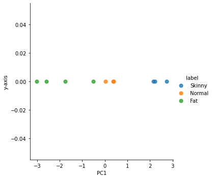
SKlearn PCA 라이브러리 이용
In [55]:
from sklearn.decomposition import PCA

pca = PCA(n_components=1)
df_pca = pca.fit_transform(X_std)
In [59]:
df_pca

result = pd.DataFrame(df_pca, columns=['PC1'])
result['y-axis']=0.0
result['label']= y_target

sns.lmplot('PC1', 'y-axis', data= result, scatter_kws={'s':50},hue='label', fit_reg=False)
C:\ProgramData\Anaconda3\lib\site-packages\seaborn\_decorators.py:36: FutureWarning: Pass the following variables as keyword args: x, y. From version 0.12, the only valid positional argument will be `data`, and passing other arguments without an explicit keyword will result in an error or misinterpretation.
  warnings.warn(
Out[59]:
<seaborn.axisgrid.FacetGrid at 0x2652b3035e0>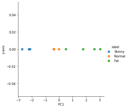
In [60]:
#### 붓꽃 데이터로 해보기 pca 2로 해보기
In [63]:
from sklearn.linear_model import LogisticRegression
from sklearn.model_selection import train_test_split
from sklearn.decomposition import PCA
from sklearn.datasets import load_iris
import pandas as pd
import numpy as np
import matplotlib.pyplot as plt
from sklearn. preprocessing import StandardScaler

iris = load_iris()
columns = ['sepal_length', 'sepal_width', 'petal_length', 'petal_width']
irisDF = pd.DataFrame(iris.data, columns=columns)
irisDF['target'] = iris.target
In [64]:
iris_scaled = StandardScaler().fit_transform(irisDF)
In [74]:
pca  = PCA(n_components=1)
pca.fit(iris_scaled)
iris_pca = pca.transform(iris_scaled)

pca_columns = ['pca_component_1']
irisDF_pca = pd.DataFrame(iris_pca, columns = pca_columns)
irisDF_pca['target']=iris.target
In [75]:
from sklearn.ensemble import RandomForestClassifier
from sklearn.model_selection import cross_val_score

rcf = RandomForestClassifier(random_state=156)

X_train, X_test, y_train, y_test = train_test_split(irisDF_pca, irisDF_pca, random_state=156)
scores = cross_val_score(rcf, irisDF_pca, iris.target, scoring = 'accuracy', cv =3)


print(scores)
[0.98 1. 1. ]728x90
'데이터 전처리' 카테고리의 다른 글
| SVD 특이값 분해 (0) | 2022.04.26 |
|---|---|
| LDA(Linear Discriminant Analysis) (0) | 2022.04.26 |
| PCA- UCI 크레딧 카드 실습 (0) | 2022.04.26 |
| 데이터 전처리-피쳐 스케일링과 정규화 (0) | 2022.04.11 |
| 데이터 전처리-data encoding (0) | 2022.04.11 |